# What do numbers look like?
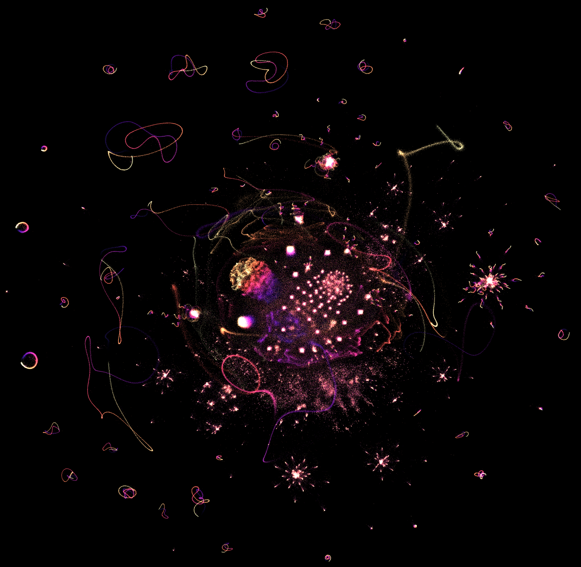
## A view of a million integers
This is the first million integers, represented as binary vectors indicating their prime factors, and laid out using the [UMAP dimensionality reduction algorithm](https://github.com/lmcinnes/umap) by Leland McInnes.
Each integer is represented in a high-dimensional space, and gets squished down to 2D so that numbers with similar prime factorisations are closer
together than those with dissimilar factorisations.
A very pretty structure emerges; this might be spurious in that it captures
more about the layout algorithm than any *"true"* structure of numbers. However, the visual effect is very appealling and requires no tricky manipulation to create.
[Large 4k version of the image suitable for backgrounds](imgs/primes_umap_1e6_4k.png)
### Code
The [python code is available](https://gist.github.com/johnhw/dfc7b8b8519aac530ac97da226c17bd5).
[Massive ~10k resolution version 16Mb](imgs/primes_umap_1e6_16k_tight_crop.png)
### Video
A short video, showing the numbers being added in sequence. Each frame adds 1000 integers,
for a total of 1000 frames.
Note that the layout is a fixed layout for 1M points, and the video shows the points in this 1M point filtered over time. It is not a recomputation of the layout
for each subset, as that would be too unstable to make a useful animation.
### Interactive 3D viewer
There is a WebGL live in-browser [3D viewer here](https://johnhw.github.io/umap_primes/three_umap.html). The algorithm was run again compressing into a 3D space, instead of 2D.
Much of the structure remains stable, which is very pleasing. This plot uses the "false colouring" to colour the points, as explained in below.
The [2D plot can be viewed as well in the same viewer](https://johnhw.github.io/umap_primes/three_umap.html?npy=1e6_pts_2d_int16.npy&color=plasma).
### I want a poster of this for my classroom/office/bathroom

There are posters from Zazzle.com here:
* [with explanatory text](https://www.zazzle.co.uk/one_million_integers_poster-228015218041429815)
* [without text](https://www.zazzle.co.uk/one_million_integers_no_text_poster-228952618305725698)
## What if we go further?
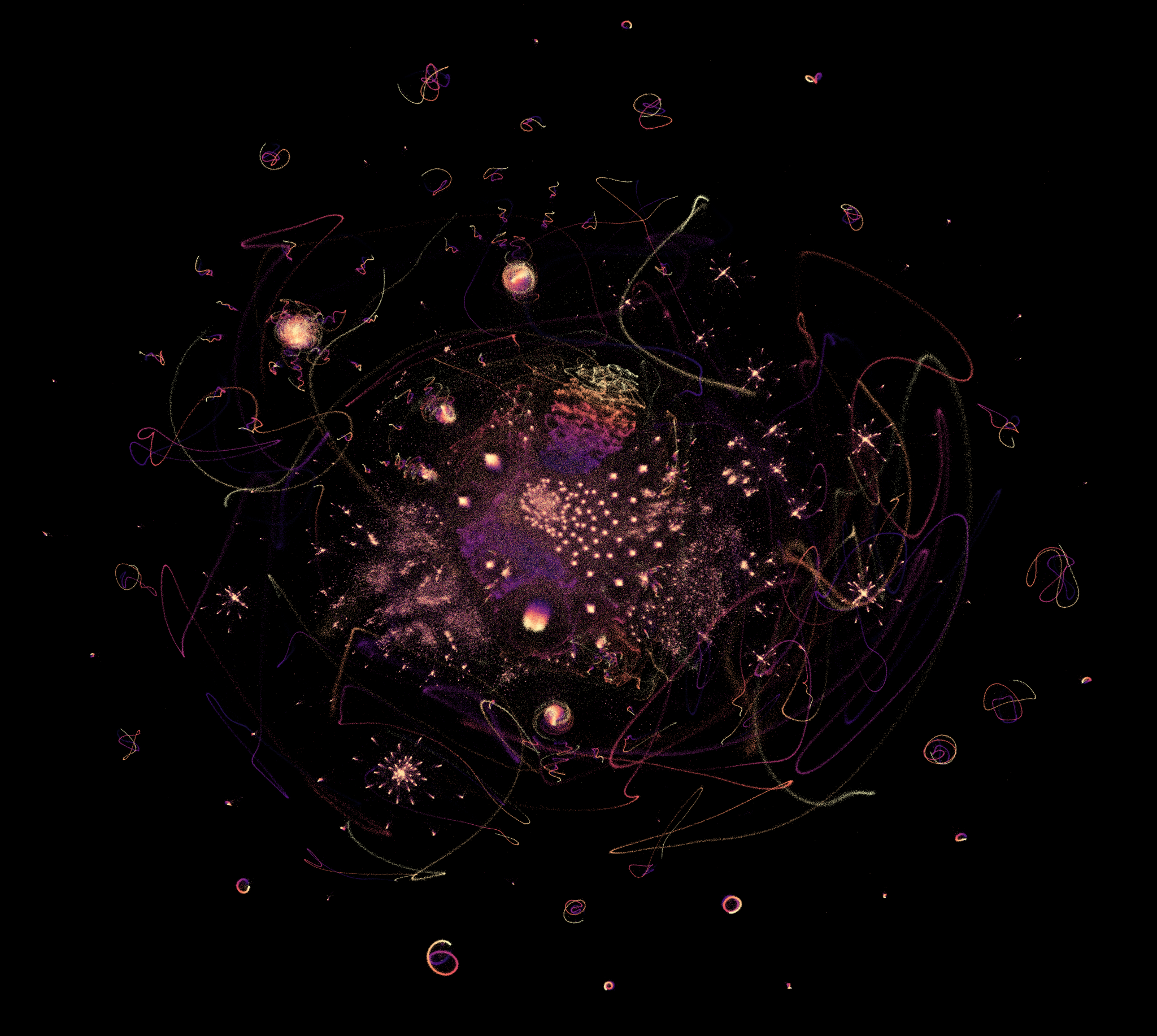
### 2 million
The image below shows the results for two million integers, with an even richer texture.
### 8 million
The image below shows the results for eight million integers, with some intense swirling threads.
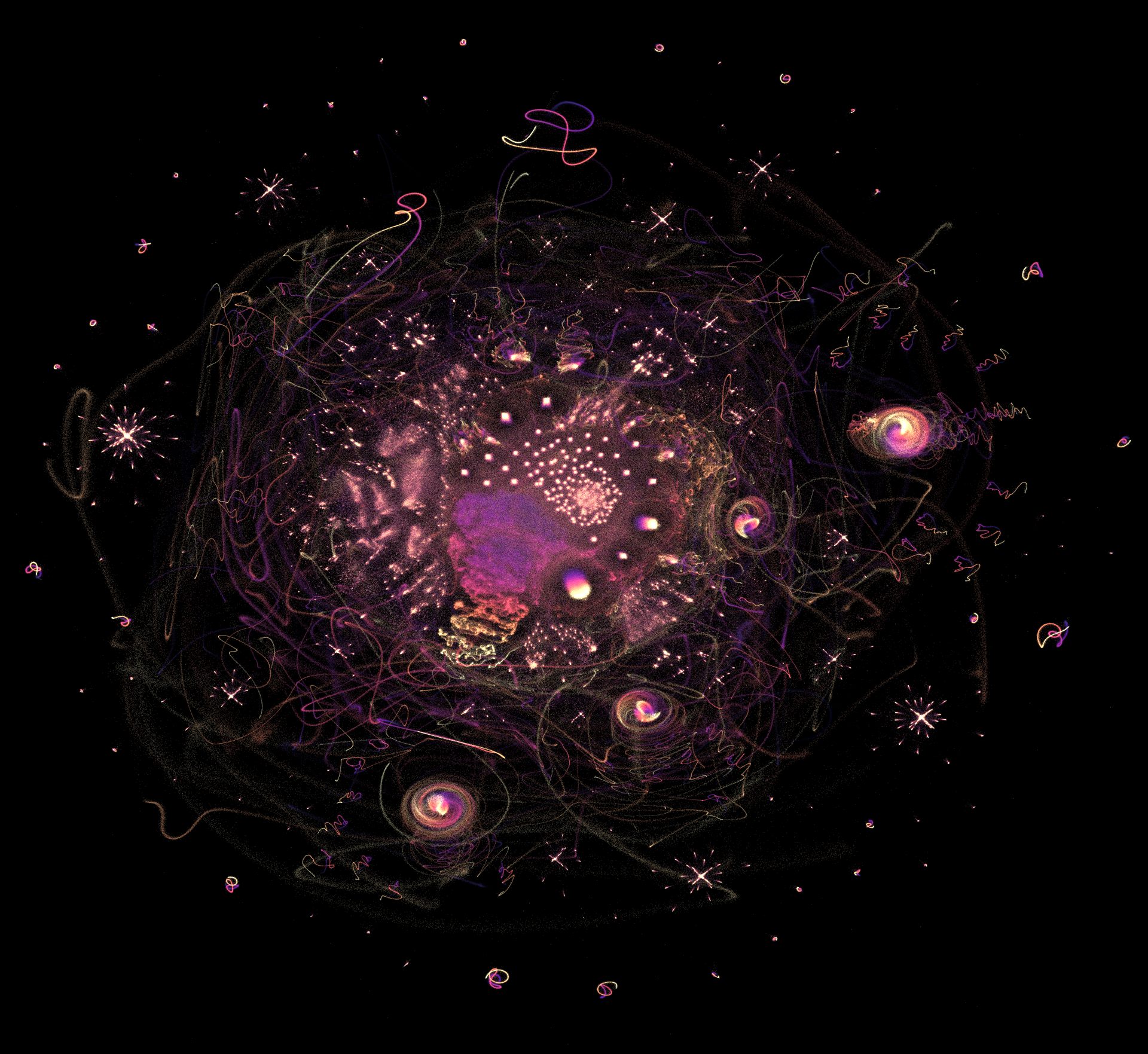
Going beyond this is restricted by available RAM, but it seems that computing layouts up to around 10-20M points should be possible.
## Representation
Each natural number can be thought of as being *composed* of a number of simple elements: the product of their prime factors. For example 50 = 5 * 5 * 2. The prime
factors are a basis ("building blocks") from which other numbers can be constructed.
In a vector space, there is a similar concept. Any vector, like the 3D vector `[1,9,2]`, can be written as a sum of *basis vectors* such as the conventional:
[1,9,2] = 1 * [1,0,0] + 9 * [0,1,0] + 2 * [0,0,1]
This visualisation links these two concepts. It *decomposes* each number into its basic components (the prime factors) and then creates a vector
with bases which correspond to each prime building block. This gives a geometry to the numbers, and we can then apply concepts such as norm (distance)
and inner product (angle) to this space. These are very high-dimensional vectors; more than 70,000 dimensions for the above image.
Each integer is represented
as a vector, one element for each possible prime factor, where 0=prime factor not present, 1=prime factor present. This provides a simple geometry for the
integers, where each number can be seen as being composed of prime basis vectors. These high-dimensional vectors are then squashed down
from thousands of dimensions for each number to just two dimensions, in a way that keeps points with common factors close together, and then a point is plotted at that 2D coordinate. The points are laid out so that numbers with similar "angles" to each other are close together. For example, all primes are at 90 degrees to each other, and all powers of a number are identical to each other (0 degree angle).
The points are coloured according to the original integer index; brighter colours correspond to larger numbers.
For example, 10 might be represented as `[1 0 1 0 0 0 0 ...]` as it has factors 2 and 5 (the first and third primes respectively). This isn't a *unique* representation,
as it represents all repeated prime factors with the same vector (e.g. `2=[1 0 0 0...]`, `4=[1 0 0 0 ...]` and `8=[1 0 0 0 ...]`, and so on for every power of 2).
### Manifolds and graphs
This means that every number is represented as a point inside (actually on the corners of) a $n$-dimensional cube, spanning `[0 0 0 ...]` to `[1 1 1 ...]`. We might postulate that these integers lie on some interesting subspace of this cube. For example, they could lie on a **manifold**, a topological structure which is locally like "normal" Euclidean space but bent and twisted into some higher dimensional space. The effect of UMAP is to try and disentangle any manifold that might exist, and "unwrap" it in a lower dimension, essentially by cutting and gluing parts of the high-dimensional space together (very loosely speaking). This is analagous to the way a 3D sphere can be approximately squashed to a plane with some gaps by cutting it into orange-wedge segments and gluing them together. In this case, the unwrapping was to two dimensions, to make it easy for humans to look at.
The manifold hypothesis is clearly very dubious for this dataset because the integers are necessarily discrete and cannot form a continuous space -- the vectors are all on the corners of a hypercube by definition! It makes no particular sense to interpolate between any of these vectors (while one could postulate an extended number system which included arbitrary interpolated elements, it would just correspond to the positive orthant of the infinite dimensional vector space over the reals, $\mathbf{x} \in \mathbb{R}^\infty, 0 \leq x_i \leq 1$, and not be especially interesting).
A better conceptual model would be a graph, where each vertex is a number, and there is an edge between every number sharing a prime factor, with edges weighted by the number of shared factors (normalised in a particular way: see below). The vector space geometry is perhaps better thought of as a convenient way of embedding this graph to define norms and perform a (relatively) smooth deformation onto the plane for display via UMAP.
### The frontier
It's worth noting that any structure that is not an algorithmic artifact is really the **frontier** of numbers at some threshold (in this case, 1 million).
*Every* possible
finite binary vector corresponds to at least one integer in this representation (actually, infinitely many, as all repeated factors are
contracted onto a single binary indicator). Therefore, in the infinite set of integers, all points are present, at every possible angle or distance from
each other, and the space would be perfectly evenly filled. However, by cutting off at some specific `n`, we see the "surface" that we have reached by composing together primes such that
their product is less than `n`. It's the specific sparsity that we get by capturing only the numbers less than some limit that brings the structure. As any binary matrix corresponds to a possibly non-unique collection of integers in this representation, any selection criterion for choosing that matrix is an implicit criterion for the numbers chosen.
It might be tempting to say that the images show "what primes look like"; but it would be more accurate to say that they show "a portrait of a million".
### Algorithm
* for each `i` up to `n`
* find prime factors of `i`.
* For each `i`, make binary vector with [`π(n)`](https://en.wikipedia.org/wiki/Prime-counting_function) columns (π(n) = number of primes less than `n`), where each element has `1`=prime factor present, `0`=absent.
* Stack all vectors into a large, sparse matrix
* Lay out with UMAP, using the cosine distance function (normalised dot product).
I used [`li(n)`](https://en.wikipedia.org/wiki/Logarithmic_integral_function) as a cheap upper bound on `π(n)` to estimate the number of columns needed.
For example, for `n=11`, the matrix looks like:
```
2 3 5 7 11
[0. 0. 0. 0. 0.] 0
[0. 0. 0. 0. 0.] 1
[1. 0. 0. 0. 0.] 2
[0. 1. 0. 0. 0.] 3
[1. 0. 0. 0. 0.] 4
[0. 0. 1. 0. 0.] 5
[1. 1. 0. 0. 0.] 6
[0. 0. 0. 1. 0.] 7
[1. 0. 0. 0. 0.] 8
[0. 1. 0. 0. 0.] 9
[1. 0. 1. 0. 0.] 10
[0. 0. 0. 0. 1.] 11
```
Each row represents one integer. Each column represents the presence or absence of the prime factor for that integer.
The image at the top is reduced from a 1000000x78628 (!) binary matrix to 1000000x2. This only works because of the excellent sparse matrix support in UMAP.
#### How does UMAP work?
If you want to know what UMAP does -- and it is the magic ingredient here -- then I thoroughly recommend the video by UMAP's author, Leland McInnes:
## What are we seeing?
The points can be filtered according to whatever criteria we might be interested in. For example, the parity of the numbers (even=green, odd=orange)

or alternatively by the whether the points are prime or not (white=prime, blue=composite).

As might be expected, the primes form the vague, diffuse cluster near the centre, as they are all orthogonal to each other.
Extending this idea, we can colour the points by number of unique factors:

We can colour the points according to the prime factors they contain, where the log of the factor is mapped to hue, with redder=smaller, bluer=larger
factor. This generalises the parity plot above. This plot has just a touch of spatial noise added to try and separate out the colours more clearly,
as each factor pass is rendered as a separate layer.

### Sequences
We can look at where common sequences of numbers lie. This isn't particularly informative, but there is perhaps some pattern.
For example, the Fibonacci sequence:

or the squares:

Colouring by sequence [A083140](https://oeis.org/A083140), the sieve of Sieve of Eratosthenes
read off in an anti-diagonal order, shows some vageu structure (but perhaps just a result of
approximate magnitude ordering).

## Reproducibility
### A random control
How much of what we see is just algorithmic artifacts, and how much is to do with the number representation? One way of getting at that question
is to rerun the layout algorithm with a similar, sparse binary matrix, but with random entries.
To test this, I created a 1000000x78628 sparse matrix with the same density of 1s as the integer representation (approx 0.24% of the values being 1) and
reran the algorithm. The result is this:

The same plasma colour map is used as in the first plot. The result **isn't** just random noise, so there clearly is some artifacting going on (or it could also
be artifacts of NumPy's random number generator, but I think that's unlikely to give the structure we see).
I am not sure what the blobby clusters represent, but they are possibly related to the count of 1s in each vector. Note, however, that the colouring
is random and diffuse, and there are no loop structures or hierarchical clusters. These seem to be a true function of the data chosen.
This does not show that what is shown is some deep truth but it provides some evidence that the result is not wholly arbitrary, along with a hint of caution that even random data can produce *some* apparent structure.
### Is this stable?
One important question arises from the stochastic nature of the UMAP algorithm: is what we see
reproducible and stable, or the artifact of one particular run of the algorithm? The results below
show ten repetitions of exactly the same data with the same hyperparameters but random initial conditions. While parts of the layout
move around (as would be expected) it is clear that the structure that is revealed remains comparable.

These images are manually
aligned so that the large cluster with the smooth gradient (highlighted with the green box in the first image)
is in the same place in each plot, for easier comparison. The rotation of the layout as produced by UMAP is arbitrary.
It should be noted that this doesn't show the effect of different hyperparameters of the UMAP algorithm.
#### Hyperparameters
UMAP is flexible and has a number of *hyperparameters* that can be configured to produce different layouts. It is wise to be cautious when using dimensional reduction algorithms, as the results can pull apparent
structure from nothing at all if configured poorly; or alternatively fail to find structure that is there.
See, for example, [How to Use tSNE Effectively](https://distill.pub/2016/misread-tsne/) on Distill.pub,
or the example [using UMAP on a Gaussian noise blob](https://github.com/lmcinnes/umap/issues/94) for cautionary tales.
UMAP has [two key hyperparameters](https://umap-learn.readthedocs.io/en/latest/parameters.html):
* **n_neighbors** which "balances local versus global structure in the data". **Default 15.**
* **min_dist** which "controls how tightly UMAP is allowed to pack points together". **Default: 0.1**
The results below show a number of runs of the 1M point layout with different hyperparameters. While there is a significant effect
of the hyperparameters, it appears that the underlying structure is fairly stable. The hyperparameters were randomly uniforms sampled
from **n_neighbours** in [3,32] and **min_dist** in [0.02, 0.95]. This gives a range of reasonable values. Fifteen variations are shown below.

UMAP has many other hyperparameters that can be tweaked, but most of them would be expected to have a relatively small effect on the final layout (though might affect the efficiency of the layout process).
##### Initialisation
The UMAP algorithm can be initialised randomly, or using a spectral initialisation algorithm. Both variations lead to virtually indistinguishable results for this dataset, though the spectral initialisation is significantly more RAM-hungry. For example, the 2M point image below was computed with random initialisation. The 1M point image at the top was computed with spectral initialisation.
# Theory
[There are some rough and unfinished notes covering empirical and theoretical analysis of what we are seeing.](theory.md.html)