# Number Spirals  ## Introduction [This is a slightly updated version of this post from back in 2009](http://www.dcs.gla.ac.uk/~jhw/spirals/) The well-known [Ulam spiral](http://en.wikipedia.org/wiki/Ulam_Spiral) and the variant developed by Robert Sacks, the [Sacks spiral,](http://www.numberspiral.com) show interesting geometric patterns in the positions of primes. This page explores a simple extension of these spirals to visualize the number of unique prime factors for each number and provides Python code for drawing them, along with some pre-rendered examples, in PostScript and PNG format. 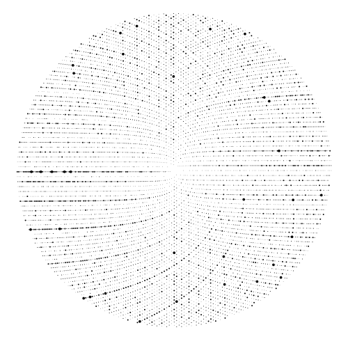## Construction The layout of the Sacks spiral aligns the squares (1,4,9,16,... etc) along a straight line heading east from the center. Its construction is very simple: the polar co-ordinates of each integer $i$ is just: \[ \theta = 2 \pi \sqrt{i} \\ r = \sqrt{i}, \] and thus its Cartesian $x,y$ co-ordinates are given by: \[x = -\sqrt{i}\cos(2\pi\sqrt{i})\\ y = \sqrt{i}\sin(2\pi\sqrt{i}) \] The result is a spiral like this:  ------------------------------------------------------------------------ ### Prime Factor Spirals In the original construction, points are coloured if they prime and uncoloured if not. Dense clustering of primes along particular paths appears. This is quite unexpected, and to an extent unexplained. 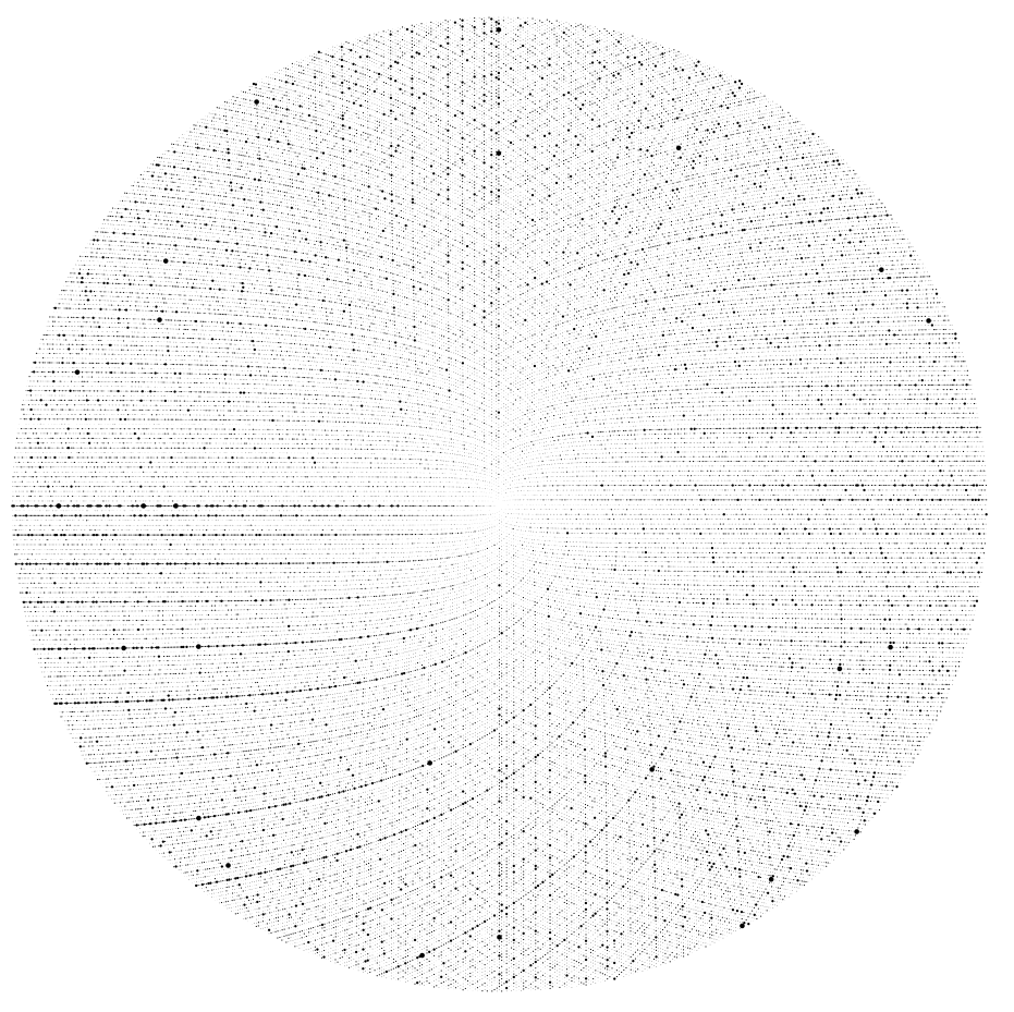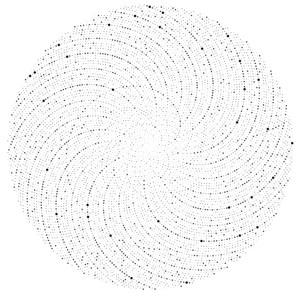By generalizing to visualize the **number of unique prime factors**, other geometric features appear. For example, the radius of each drawn circle can be made proportional to the number of unique prime factors the associated number has. The result is an extremely rich and varied pattern.  This is an image of the first 10000 numbers laid out in such a spiral, produced by the Python code given below. Why unique prime factors? Well, it seems to have a lot of visual structure -- more interesting than the same plots showing total prime factors, or other variations. It's easy to plot variations if you feel like exploring them; after all the code you need is all here. ### Interesting Features -- A Short Tour There are a number of geometric features that appear on the plots. 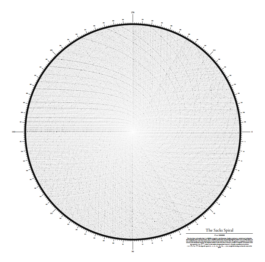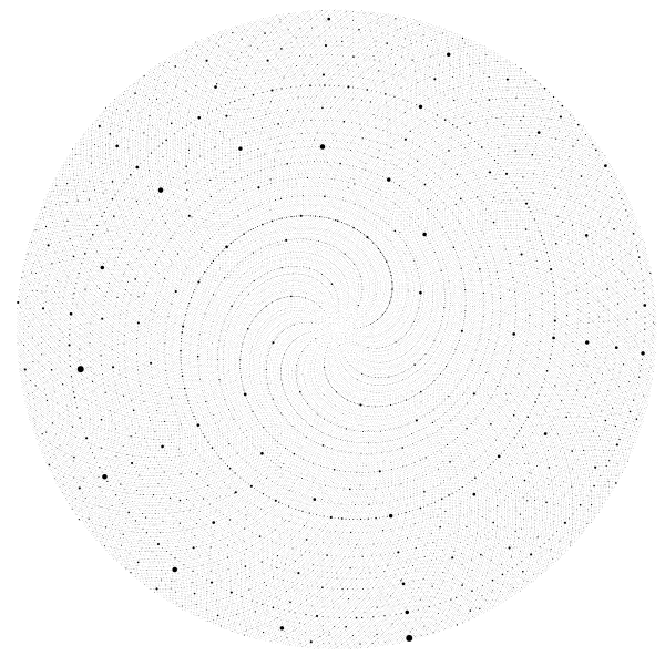To see most of these features, we need to look at a high-resolution image of the spiral with at least 100,000 points. The [big PNG version (6600x6700px)](imgs/spiral_1e5_full.png) has sufficient detail.  All of the angle references apply to the compass drawn around the 100,000 point version. **The sparse curves.** There are several curves which are very sparse (i.e. there is a high density of prime numbers and few-factored composites). The most prominent of these meets the exterior at about 203 degrees. A second, smaller one meets the exterior at 189.5 degrees. Another meets at 37 degrees and has a fainter parallel at 29 degrees. **The vertical lines.** Between about 90 and 70 degrees, and between 270 and 250, there are distinct, unevenly spaced vertical lines, getting more tightly spaced as the axes (90 and 270) are reached. **The diagonals.** At exactly 60 and 300 degrees two fuzzy lines extending from the center are clearly visible. A number of fainter parallel lines can be seen, anti-clockwise from the original lines. A symmetric pair at 120 and 240 are very faintly visible. **Dense horizontals.** In the quadrant from 90 to 180 degrees, numerous dense lines can be seen, becoming more tightly spaced towards 180 degrees. The line at exactly 180 degrees is the densest line on entire spiral. ------------------------------------------------------------------------ ### Code The code for generating rendering the spirals is very simple. For maximum quality, a vector format is desirable; I've used [PyX](http://pyx.sourceforge.net/) package to render to PDF. ### Pre-requisites To run these examples, you need Python, [PyX](http://pyx.sourceforge.net/), and the elementary number theory package [ent.py](src/ent.py) by [William Stein](http://modular.fas.harvard.edu/ent/). Both of these are pure Python and should run on any platform. #### Basic version The simplest code looks like this (this produces the image of the first 10000 points shown earlier): ```python from pyx import canvas, document, path from ent import factor from math import sin, cos, sqrt, pi n = 10000 ca = canvas.canvas() for j in range(n): i = j + 1 r = sqrt(i) theta = r * 2 * pi x = cos(theta)*r y = -sin(theta)*r factors = factor(i) if(len(factors)>1): radius = 0.05*pow(2,len(factors)-1) ca.fill(path.circle(x,y, radius)) d = document.document(pages = [document.page(ca, paperformat=document.paperformat.A4, fittosize=1)]) d.writePDFfile('spiral_1e4.pdf') ``` [spiral_1e4.py](src/spiral_1e4.py) The PDF file generated is [spiral_1e4.pdf](pdf/spiral_1e4.pdf). This could easily be changed to color the points differently instead of modulating the radius, e.g. by replacing the ` ca.fill() ` call with ```python ca.fill(path.circle(x,y, 0.3), color.palette.RedGreen.getcolor((len(factors)-1)/8.0))) ``` There are lots of visualisation techniques that could be used -- for example false colouring the image using one color channel for the number of unique factors, one for the primes, and another for the total number of factors. If you find any interesting ones, please let me know. In this code, the radius of each point is $2^{f-1}$ (where $f$ is number of unique prime factors). Prime numbers are omitted entirely. The exponential scaling is largely arbitrary; I tried a number of different functions and found this to be the most revealing. Since numbers with large numbers of unique prime factors are rare in small integers (no number below 9699690 can have more than seven), the mapping works well. #### Scaling Up The output for 100,000 points is [spiral_1e5.pdf](pdf/spiral_1e5.pdf).  [spiral_with_labels.py](src/spiral_with_labels.py) adds a compass (divided into tenths of degrees) around the utside of the area, and adds a textual label. NOTE: If you're using this code, you'll either need to have LaTeX installed to do the text rendering, or comment out the "texrunner" lines from the source in `write_label()` and `draw_axis()`, and live without the labels. For 1,000,000 points the extremely dense result is shown below (you'll have to run it yourself if you want the 178M PDF file!)  I've rendered up to 10,000,000 points successfully with this code. However the files are huge and slow, so if you want to see you'll need to render it yourself! ### Vogel Spiral Using [Vogel's floret model](http://en.wikipedia.org/wiki/Fermat%27s_spiral) for layout also gives nice results. This model gives each integer i polar co-ordinates: $$ r = \sqrt{i}\\ \theta = \frac{2\pi i}{\phi^2} $$ where $\phi$ (the golden ratio) is given by: \[ \phi = \frac{1 + \sqrt{5}}{2} \] The result of this arrangement is to align the Fibonacci numbers along the eastern axis (although the first few are slightly off axis).  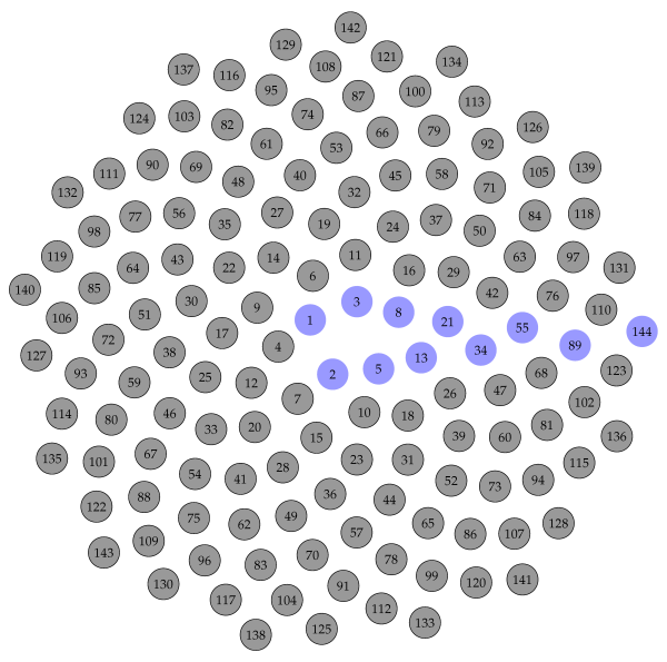In contrast to the original spiral, which had a square on every turn, the spacing between Fibonacci numbers increases rapidly. The above image was generated by [vogel_labeled.py](src/vogel_labeled.py).  [spiral_vogel_1e5.pdf](pdf/spiral_vogel_1e5.pdf) is the 100,000 point PDF. This unadorned spiral was generated with [spiral_1e5_vogel.py](src/spiral_vogel.py) . 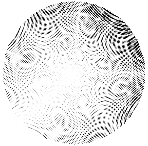The Vogel spiral has quite a different pattern when plotting the total number of factors rather than the number of unique ones (100,000 point plot). In fact, if the Vogel spiral plots of the total and unique factors are overlaid, they show very little visual relation to each other.  The python source that generates this image is [spiral_vogel_all.py](src/spiral_vogel_all.py) , and the PDF is [pdf/spiral_vogel_all.pdf](pdf/spiral_vogel_all.pdf). #### Fibonacci sums A quick aside: every integer can be represented a sum of one or more distinct Fibonacci numbers. Some numbers cna be represented only one way (e.g. the Fibonacci numbers themselves), while others can be represented in multiple ways (e.g. 8=8, 8=5+3 and 8=5+2+1). The number of ways a number can be represented is notated H(n), and is Sloane sequence [A0000119](http://www.research.att.com/~njas/sequences/?q=a0000119&language=english&go=Search) . 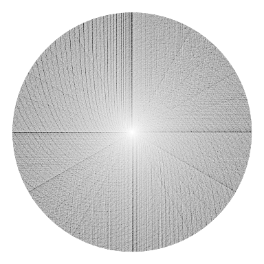Plotting this function on the Vogel spiral is easy: [spiral_nfib.py](src/spiral_nfib.py)  ## Direct Rasterization Above 1M points, producing lossless vector files is too inefficient to be very useful. Instead, the points can be directly rasterized onto a grid as they are computed, and a grayscale bitmap output file created. Using a simple antialiased pixel rendering technique (Wu pixels) avoids aliasing as the image is built up. I've done renders up to 100,000,000 point using direct rasterisation on a 4096 x 4096 grid. The image below shows a 100,000,000 point render.  [John H Williamson](https://johnhw.github.io) [GitHub](https://github.com/johnhw) / [@jhnhw](https://twitter.com/jhnhw)